
Octave
Octave is an open source alternative to MatLAB, and a powerfull software to work with big data files. Its process time for the operations are much faster compared to other tools such as spreadsheet softwares. Different packages are available, depending on the users needs, but for several applications a basic version of the software is enough, as it allows matrice operations, data filttering, fitting to experimental data, and more.
In this manual we present only an introduction to minimal data processing. A detailed description of all of its capabilities would be too extense, and out of the scope of this work. Our goal is then to familiarize the user with Octave enviroment, and how to use it to simple data preparation for plotting using Gnuplot software, available in the second part of this manual.
Octave is an open source software that can be downloaded from the homepage: https://www.gnu.org/software/octave/
1. Octave basics
We can start octave in two ways: on a terminal window (Octave CLI) or with an integrated graphics interface (Octave GUI). This manual is focused on this last one.
1.1. Working area layout
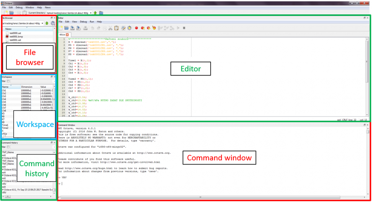
Octave GUI can be accessed on the start menu of your computer. When you initialize it, it opens a window that is divided into five separate parts. This standard layout can be personalized by the user. The next figure shows an example of this window, with the functions of each of its parts.
In the file browser, the files can be selected and opened. The workspace shows a list of all generated matrixes and their parameters. The editor is where the script is written, changed, and run. The command can be written in the command part, where we can also copy and paste parts of the script to test it, or run fractions of the script. Here you can also access the help menu by writing "help command" that will show us information about that command, or function. The last part of octave area is the command history window that shows all previous commands.
1.2. Saving and running the script
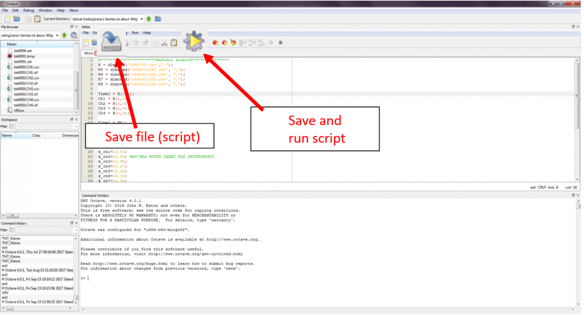
To save a script we can use the icon highlighted in the next figure on the left. The scripts for octave are saved with .m extension. To run a script we can use the highlighted icon in the right or we can copy the script (or part of it) and paste it on the command window.
1.3. Opening a saved script
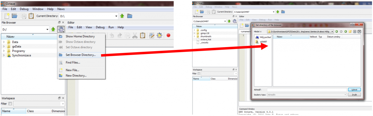
If we already have a script saved on our disc, we can open it by setting a path to the folder containing the script and then confirming it, as shown in the next figure.
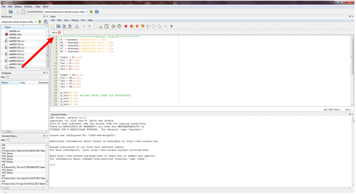
The folders and scripts will be now shown in file browser. To be able to work with the script we can double-click it, and it will be opened in the editor, as shown in the figure below.
2. Loading a data file
Octave can read different types of data files (.txt, .csv, .dat) and also binary files and pictures. We can use dlmread or load functions to load the datafiles. Aditional options can be added to the funcions, as described in following examples.
Command and options description:
X = dlmread ('XXX.csv', " ", [0, 0, 50000, 2]);
Name of loaded matrix:
- X =
Command for data file loading:
- dlmread()
Name of data file loaded from the disc:
- 'XXX.csv'
Colum separator used in data file (in this case a space):
- " "
Data limits for reading. From left to right, First line, first column, last line, last column. In this example, lines from 0 to 50 000 will be loaded from columns 0 and 1.
- [0, 0, 50000, 2]
Example:
CH1 = load('Shot1_CH1.csv');
- CH1 =
Name of the matrix (e.g. CH1 as a channel 1)
- load()
Command for data loading
- "Shot1_CH1.csv"
Name of data file, as saved on the disc.
2.1. Working with data file collums separetelly
If we need to work with the datafile columns separately (or as vectors) we can first load the datafile to a matrix called e.g. "X" (see the previous topic), and then divide the matrix X into separate columns by the following commands.
Example:
Time = X (:,1);
ch1 = X(:,2);
In this example, the first collum of the data file (and of matrix X) is the time, and the second collum is the variable measured in ch1. The first command then loads only the first collum of matrix X into a new matrix called „Time“. The same is done for the second column, that is loaded into the matrix called „ch1“.
Name of a new matrix: „Time“:
- Time =
Name of the matrix with the original data. In the brackets, we can select which lines are going to be loaded in that column (in this example, column 1).
- X(:,1);
- : – All lines
- 1 – First column
3. Basic operations
In this chapter, we show how to define basic mathematical operations as addition, subtraction and multiplication by a constant. This operation can be useful for changing data units (eg from m to mm) or for converting raw signals to the variable of interest, by recalculation with a calibration constant.
3.1. Basic mathematical operations
As in regular matrix operations, the size of the matrix has to be taken into consideration. E.g. addition and subtraction of two matrixes require that they have the same dimensions. The regular dimension compatibility for multiplication and division apply.
Summing matrices x and y:
- x + y
Subtraction of matrix y from matrix x:
- x – y
Multiplication matrix x by matrix y:
- x * y
Division matrix x by matrix y:
- x / y
Sign inverting:
- -x
The square root of matrix y:
- x=sqrt(y)
Complete example:
X = dlmread("matrix1.csv",";");
Y = dlmread("matrix2.csv",";");
Z = X + Y;
In the first step, the X and Y receive the data from the files matrix1 and matrix 2. Then the loaded matrices are added, obtaining matrix Z. The addition is shown in the following table.
| Matrix 1 | Matrix 2 | Result | ||||||||
| 1 | 1 | 1 | + | 2 | 2 | 2 | = | 3 | 3 | 3 |
| 2 | 2 | 2 | 2 | 2 | 2 | 4 | 4 | 4 | ||
| 3 | 3 | 3 | 2 | 2 | 2 | 5 | 5 | 5 | ||
The data files used for this example can be downloaded here as a .csv files: matrix1 and matrix 2.
3.2. Mathematical operations element by element (Dot operations)
In Octave, we can also multiply/ divide the matrixes by a constant. In this case, every element of the matrix will be multiplied/ divided by this constant.
We can also do the multiplication element by element in the matrixes, and in this case, the elements in corresponding positions of each matrix are multiplied. A "Dot“ before the multiplication or division sign indicates that that operation is element by element, and not matrices operation.
- x.* y
multiplication element by element. E.g. for (1 2 3).*(4 5 6) the result will be calculated by (1*4 2*5 3*6)
- x./y
division element by element
- x. – y
subtraction element by element
- x.^y
matrix x powered element by element (or by constant if y has fixed value)
In this example, we will demonstrate the multiplication of a matrix by a constant. The first step is to define the constant. Then the matrix can be multiplied by this constant by writing .* (multiplication sign with the dot) and the matrix name. In the example, we have the constant k_ch1 (in kPa/volts) as being a calibration constant, and the signal loaded in the matrix ch1(in volts) is multiplied by this constant to get the converted matrix ch1p(in kPa).
Examle:
k_ch1 = 13.54;
ch1p=ch1.*k_ch1;
Constant name:
- k_ch1
Constant value:
- = 13.54
Name of the recalculated matrix (e.g. channel 1 recalculated to pressure):
- ch1p
Multiplication of matrix ch1. The dot means multiplication element by element. Unlike in the standard matrices multiplication, matrix dimensions always remain the same:
- ch1.*
Previously defined constant by which the matrix ch1p will be multiplied:
- k_ch1
3.3. Loop function "for"
A loop can be used if we need to repeat one or more operations. To start the for command we need to define the number of cycles and the operations. The command end closes the loop.
Example:
for i=1:5
x(i)=10*i;
end
In this example, the numbers 1, 2, 3, 4 a 5 are multiplied by 10, and the resulting matrix X contains the following elements: 10, 20, 30, 40 and 50.
3.4. Condition if
The if function states a condition to following commands, as shown in the following example.
Example:
if x>y
z=10;
else
z=5;
end
In this example, if the x value is bigger then y, then z is equal to 10. Otherwise, case z = 5.
4. Advanced mathematical operations
4.1. Numerical integration
The numerical integration can be done using a loop with the function for. However, in Octave a pre-defined function cumtrapz provides the same result with much less process time.
Example:
i1 = cumtrapz(Time,ch1p);
Name of the matrix containing the integrated values:
- i1
Function for integration:
- cumtrapz
Data chosen for integration. Time is on the x axis and ch1p – (in this example, pressure values) is on the y axis.
- (Time, ch1p)
4.2. Fitting to experimental data
4.2.1. Linear and polynomial fit
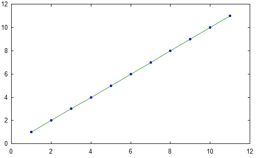
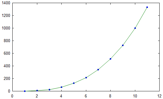
In Octave a same function for linear and polynomial fitting can be used. The following command shows a function for both linear and polynomial fitting. The values of Time-distance dependance are fitted by a second order polynomial where the number in the end of command determines the order. For a linear fitting "1" can be used.
- p = polyfit (Time, Distance, 2);
The polyfit command give us only the parameters of fit. However, for plotting of this fir we have to generate points based on these parameters. For this purpose a function polyval exists. It will generate a point for every line in "Time" matrix based on the matrix "p" generated by polyfit.
- fit = polyval(p, Time);
Command to plot the fit as two curves. One with experimental points and second as its fit.
- plot (Time,Distance,".", Time, fit);
To show a fit paremeters polyout command can be used:
- polyout(p, 'x');
Calculation of R2:
- R = corr (Time, Distance);
- R2 = R^2
|
Linear fit based on mentioned commands |
Fiiting of a points by the third order polynomial. |
5. Saving the data files
Octave has all matrices saved in cache memory. To save a matrix as a file we have to write a command, as shown in the following example.
Example:
XXX = [Time ch1p ch2p ch3p ch4p];
save -ascii "shot1.txt" XXX;
- [Time ch1p ch2p ch3p ch4p]
saving the matrix as a text file in ascii format:
- save -ascii
name of new created data file:
- "rana1.txt"
matrix that should be saved:
- XXX;
Based on the example the matrix called "XXX" will be saved as "shot1.txt" file. The first column in the file is time and the 2-5th columns contain the overpressures ch1p to ch4p. The saved data file has then five columns and uses a space as collumn separator.
6. Plotting
It is possible to create plots in Octave, what can be usefull for a quick view of results. For advanced plotting though is better to prepare the data in Octave and then create a graph in Gnuplot.
Example:
plot(Time(1:A:end,1),ch1p(1:A:end,2).-10, ";PCB;"
Setting an axes labels
- xlabel ('Time [ms] ');
- ylabel ('Pressure [kPa] ');
Setting a grid on:
- grid on;
Definition of decimation factor. If used, every Xth point will be plotted.
- A=10;
Plotting function:
- plot
Data on x axis. "1" means from the first line, A is decimation factor (every Ath point), end means to the last line and ",1" defines the column that is being read.
- (Time(1:A:end,1)
Data for y axis. Second column from matrix ch1p from the first line to the end with one every Ath line plotted.
- ch1p(1:A:end,2)
Shiftting the curve on y axis by 10:
- -10
Name of the curve:
- ";PCB;"
